Chapter 11 Applied Stats Model II Lecture Note
11.1 List of Questions:
11.1.3 Midterm
Q1: ??? #the intercept is 3.5 #??? does the intercept needs the log?
GammaPoisson - why contains no 0s? -> only probability. unless I set a cut-off point.
ICC random variance/ total variance.
why specify the mean = mean() in summarise. duplicate –> creating a variable name
Q7c: # Convert back to glm() style object ??? why needs a conversion?
# why alternative style reached? # is it the aggregated model vs. individual count? or the same???
Q7a # then why the 70 and 60 combination has service???
Q7f: #??? why is the actual data 10% 0, but here is 4.5%? Diff so much
11.2 Class content overview:
Textbook: Extending the Linear Model with R, Second Edition, 2016 by Julian Faraway
Topics: • Generalized Linear Models – Models for Proportional data. – Models for Count data. – Models for Positive continuous data.
• Mixed Models – Random Effects – Linear Mixed Models – Generalized Linear Mixed Models – Repeated Measures – Longitudinal Data
• Dependent Data – Spatial Dependence. – Spatial Point Patterns. – Time Series.
• Nonlinear Models – Neural Networks – Deep Learning
11.5 GLMs_AdvancedTopics_SP2022
data(quilpie,package = "GLMsData")
quilpie$Phase <- as.factor(quilpie$Phase)
#head(quilpie,3) |> DisplayTable
#library(tweedie)
#Rain_TW_P <- tweedie.profile(Rain ~ Phase,
#p.vec = seq(from=1,to=3,by=0.01),
#do.plot=TRUE, data=quilpie)#rain_Tweedie <- glm(Rain ~ Phase, data=quilpie,
#family=tweedie(var.power=Rain_TW_P$p.max,
#link.power=0))
#coef(summary(rain_Tweedie))#Phases <- data.frame(Phase = factor(c(1, 2, 3, 4, 5)))
#mu.Phases <- predict(rain_Tweedie, newdata=Phases,type="response")
#p_MLE <- Rain_TW_P$p.max #tweedie profile
#phi_MLE <- Rain_TW_P$phi.max #phi? -> dispersion para
#Prob_Zero_Model_orig <- exp(-mu.Phases^(2 - p_MLE)/(phi_MLE*(2 - p_MLE))) # probability of it being 0. prob of observe rain + how much rain.
#??? quilpie %>% group_by(Phase) %>% summarize(prop0_dat = mean(Rain==0)) %>% cbind(Prob_Zero_Model)#summary(Prob_Zero_Model_orig)#PoiGamPred |> round(4) |> DisplayTable
#https://stackoverflow.com/questions/67744604/what-does-pipe-greater-than-mean-in-r11.6 MM-RandomEffects_Spring2022
random effect:
not interested in specific level. vs. fixed effect - not individual slope? dummy interaction with the focal variable.
fixed effect test the mean vs. random effect test the variance (not interested in particular mean, want to see if mean actually varied across levels). ??? S11: variance depends on the random effect but mean is not affected?
P14: reading the box plot. mean, median, range??? P15: what’s the n? What’s the Sum Sq?
P21: shift in the mean vs. variance and mean 0. how do I know how much the mean is shifted???
data(pulp, package="faraway")
plot(y=pulp$bright, x=pulp$operator,xlab = "Operator", ylab = "Brightness")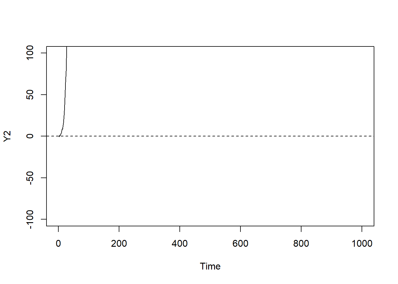
lm_model <- lm(bright ~ operator, pulp)
anova(lm_model)
## Analysis of Variance Table
##
## Response: bright
## Df Sum Sq Mean Sq F value Pr(>F)
## operator 3 1.34 0.44667 4.2039 0.02261 *
## Residuals 16 1.70 0.10625
## ---
## Signif. codes: 0 '***' 0.001 '**' 0.01 '*' 0.05 '.' 0.1 ' ' 1Prediction for each operator is simply the sum of fixed and random effect = BLUP??? components. -> S24: not in the data. new operator will take a 0 in intercept change? but the intercept can be predicted with the Xs??? -> yes, if there is blocking. how is the blend different from the operator as blocking? discrete vs. continuous?
S30: how does it match? shouldn’t it be mean + the BLUPS???
S34: fixed are irrigation that is interest. field randomly = replications?
Blocking
Split plot
Nested effect vs. random effect?
Residual plots
General: interaction terms = depends. must happen when sth happen then interaction.
11.6.1 HW4: Repeated measure, time and space dependence.
how to make R markdown slides???
11.6.1.1 repeated measure and longitudinal data / growth model/ panel study a person answers multiple questions/
All coding is simply the lanaguage the machine can understand. Succinct enough.
S4: variance may be correlated. when the variance is not multiple by a identify matrix. it means variance can correlate within group or the auto-correlation in a mini time series.??? how did the assumption change in repeated measure vs. regular group based random effect?
\(y_{i}|\gamma_{i} = N(X_{i}\beta + Z_{i}\gamma_{i},\sigma^{2}I)\) ??? how to type the ~?
S8: what’s the I(year - 68) , I() used for special ops??? S9: What’s year_fm_s | person , every person has a different slope on the year S13: not fit well??? why switch example? how to tell the tail. fat tail? S18: fortify.merMod ???
11.6.1.2 Time and Space dependence
S3: without group correlation. how to calc besides variance? two obs corr???
data(lap, package = "astsa")
plot.ts(lap[,"tempr"]) #built in function, ts time series. lap data's tempr column. 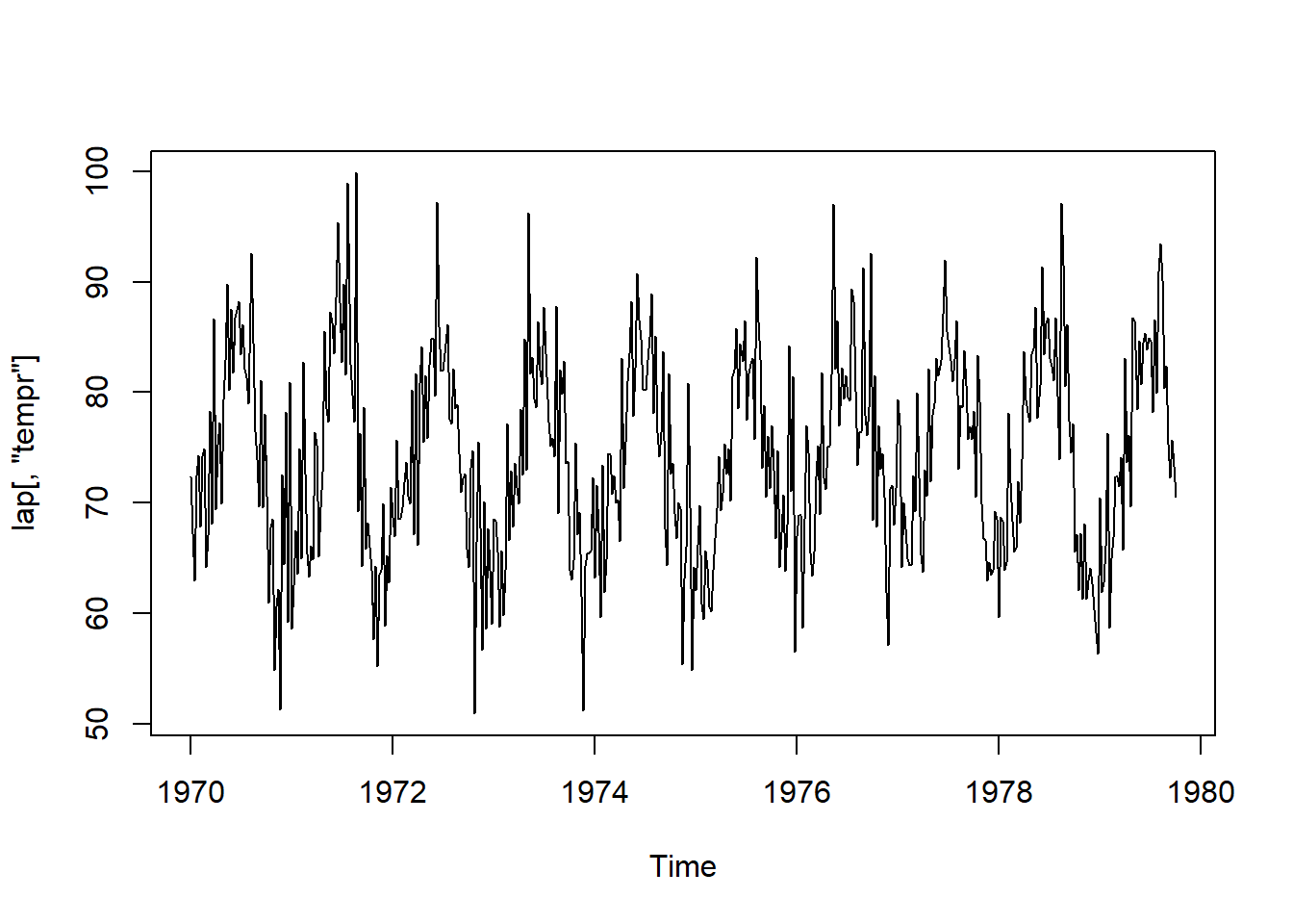
S9: stationary = no shfit in the time series. Simple seasonlity. as long as same distance aprt, the correlation will be the same.
S10: detrend using what as the base? what’s the 0 here? 12 weeks = 3 months. roll = 0/ what does it mean ???
time_lm <- lm(lap[,"tempr"] ~ time(lap)) #??? what's time() function
time_lm_resid <- resid(time_lm) # residuals of lm will "detrend"
acf(time_lm_resid) #??? what's acf? why show only 25 weeks not 52 weeks for the seasonality???
data(JohnsonJohnson)
JJ<- JohnsonJohnson
plot.ts(JJ)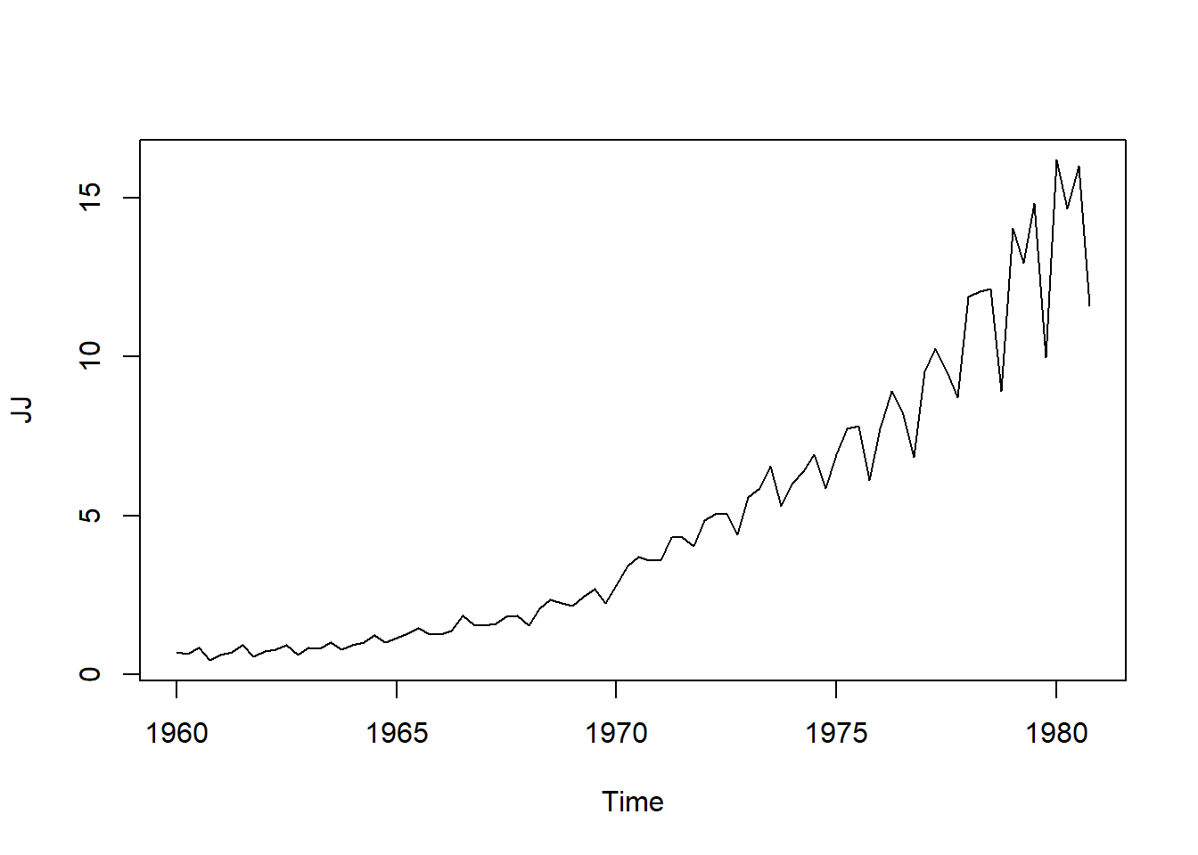
JJlog <- log10(JJ)
time_lm_JJ <- lm(JJlog ~ time(JJlog)) #???
par(mfrow=c(1,2))
plot.ts(JJlog)
abline(time_lm_JJ, col="red", lty=2)
acf(resid(time_lm_JJ))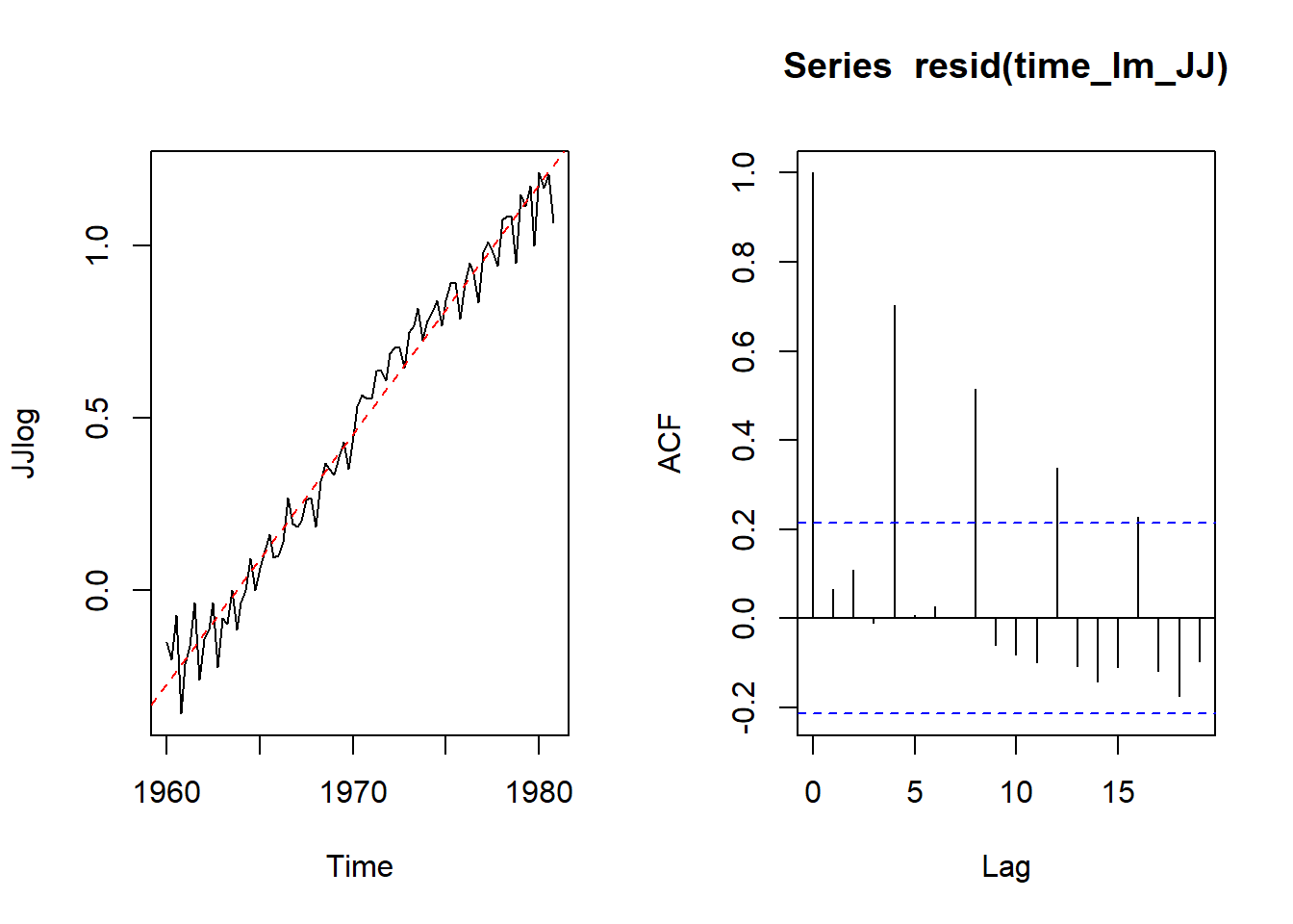
S12: how you know the seaonality. the correlation happen at the same time/location each time.
set.seed(1); n <- 50; eps_t <- rnorm(n, sd = 5)
Y1 <- Y2 <- Y3 <- double(n) #??? what's this?
Y1[1] <- Y2[1] <- Y3[1] <- 0
# Y_t = phi * Y_(t-1) + eps_t
for(i in 2:n) Y1[i] <- .75 * Y1[i-1] + eps_t[i]
for(i in 2:n) Y2[i] <- 0.1 * Y2[i-1] + eps_t[i]
#for(i in 2:n) Y3[i] <- (-.8) * Y3[i-1] + eps_t[i]
for(i in 2:n) Y3[i] <- (2) * Y3[i-1] + eps_t[i] #exploded the graph.
plot.ts(Y1,ylim = c(-15,100)); lines(Y2, col="red"); lines(Y3, col="blue")
#plot.ts(Y1,ylim = c(-15,30)); lines(Y2, col="red"); lines(Y3, col="blue")
abline(h=0,lty=2)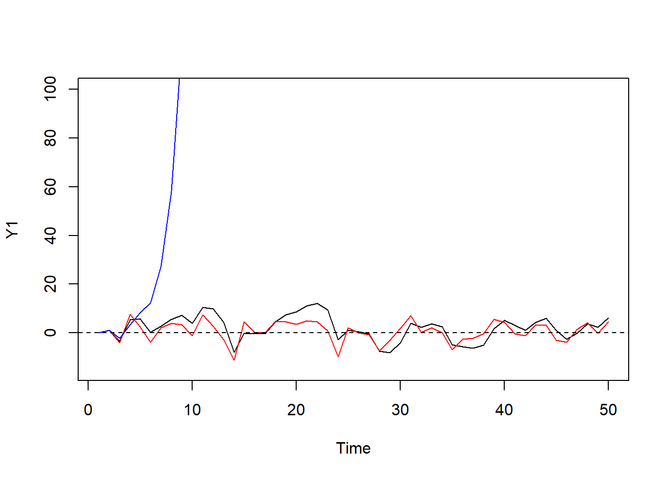
#??? blue and black should revserse but similar?S16: it has moving average only, error only???
Y4 <- Y5 <- double(n); Y4[1] <- Y5[1] <- 0
for(i in 2:n) Y4[i] <- eps_t[i] + .95*eps_t[i-1] #??? how does the program know the error? what diff between obs vs. error corr?
for(i in 2:n) Y5[i] <- eps_t[i] + .1*eps_t[i-1]
plot.ts(Y4); lines(Y5,col="red")
S18: what’s order = c(1,0,1)??? what’s p q? parameter for AR vs. MA.
Y6 <- double(n); Y6[1] <- 0
for(i in 2:n) Y6[i] <- .5 * Y6[i-1] + eps_t[i] + .4*eps_t[i-1]
lm_resids <- resid( lm( Y6 ~ I(1:n) ) )
# p q
arima(lm_resids, order = c(1, 0, 1))
##
## Call:
## arima(x = lm_resids, order = c(1, 0, 1))
##
## Coefficients:
## ar1 ma1 intercept
## 0.3207 0.5509 0.0564
## s.e. 0.1622 0.1240 1.2733
##
## sigma^2 estimated as 16.06: log likelihood = -140.76, aic = 289.51dt <- diff(time(lap))[1] # differences between time points
time_steps <- max(time(lap)) + (1:52)*dt # Time points we will predict at ??? what's the multiplication
ARMA_p1q1 <- arima(lap[,"tempr"], order = c(1,0,1))
ARMA_p1q1_pred <- predict( ARMA_p1q1, n.ahead=52 )$pred
plot.ts(lap[,4],xlim = c(1970, 1981))
lines(x = time_steps, y = ARMA_p1q1_pred, col="red") S22: ??? how do we know the correct parameter (13 8 1)?
S23:partial autocorr???
S22: ??? how do we know the correct parameter (13 8 1)?
S23:partial autocorr???