Chapter 12 STAT 4520/7520 - Homework 3 Spring 2022 Due: March 30, 2022

12.1 1) The cake dataset in the lme4 package contains data on an experiment was conducted to determine the effect of recipe and baking temperature on chocolate cake quality. Fifteen batches of cake mix for each recipe were prepared. Each batch was sufficient for six cakes. Each of the six cakes was baked at a different temperature which was randomly assigned. As an indicator of quality, the breakage angle of the cake was recorded.

Note: temperate randomly assigned. receipt, batches/replicate are nested in receipt!!!

It contains the variables: • replicate: batch number from 1 to 15 • recipe: 3 Recipes, A, B, and C • temperature: temperature at which cake was baked: 175C 185C 195C 205C 215C 225C • angle: a numeric vector giving the angle at which the cake broke. • temp: numeric value of the baking temperature (degrees F). The data can be loaded with the command.

data(cake,package = "lme4")

Additionally, we will only use the numeric version of temperature.

#library(dplyr)
#library(tidyverse)
#??? Why negative before the temperature. what does it mean?
cake <- cake |> dplyr::select(-temperature)

12.1.1 a. Of the explanatory variables recipe, temp, and replicate, which are fixed and which are random? Explain. Is there any nesting in these variables?

The recipe and Temp are fixed, since I am genuinely interested in their different levels. Replicate are random, since it is random sample of levels. I don’t care about the different replications.

The replicate/batch is nested within the recipe.

# random affect has nothing to do with random assignment in actual???
# S39: egg example, is the sample nested within technician? further split GH into G1 G2? not sure what it means. How about here is the temperature also nested??? when is it not nested? the sample are distributed across technician??? or technician switch between labs?

12.1.2 b. Fit a linear model with no random effects for breaking angle against the interaction between recipe and temperature. Which variables are significant? What is the t value for temp the temperature variable? What is the RMSE of this model?

lm_model <- lm(angle ~ recipe*temp, cake)
summary(lm_model)

## 
## Call:
## lm(formula = angle ~ recipe * temp, data = cake)
## 
## Residuals:
##     Min      1Q  Median      3Q     Max 
## -15.759  -5.279  -1.448   3.019  27.505 
## 
## Coefficients:
##               Estimate Std. Error t value Pr(>|t|)   
## (Intercept)   2.379365   9.656850   0.246  0.80557   
## recipeB      -3.649206  13.656848  -0.267  0.78952   
## recipeC      -1.941270  13.656848  -0.142  0.88707   
## temp          0.153714   0.048109   3.195  0.00157 **
## recipeB:temp  0.010857   0.068037   0.160  0.87334   
## recipeC:temp  0.002095   0.068037   0.031  0.97546   
## ---
## Signif. codes:  0 '***' 0.001 '**' 0.01 '*' 0.05 '.' 0.1 ' ' 1
## 
## Residual standard error: 7.795 on 264 degrees of freedom
## Multiple R-squared:  0.1159, Adjusted R-squared:  0.0992 
## F-statistic: 6.925 on 5 and 264 DF,  p-value: 4.285e-06

anova(lm_model)

## Analysis of Variance Table
## 
## Response: angle
##              Df  Sum Sq Mean Sq F value    Pr(>F)    
## recipe        2   135.1   67.54  1.1117    0.3305    
## temp          1  1966.7 1966.71 32.3709 3.377e-08 ***
## recipe:temp   2     1.7    0.87  0.0143    0.9858    
## Residuals   264 16039.4   60.76                      
## ---
## Signif. codes:  0 '***' 0.001 '**' 0.01 '*' 0.05 '.' 0.1 ' ' 1

The temperature variable is significant. The t value is 3.195 The RMSE is 7.79487, the MSE is 60.76

sqrt(60.76)

## [1] 7.79487

12.1.3 c. Fit a mixed model to the data which takes into account the replicates of the recipes. Examine the variance components. Is there variation in the batches made with each recipe? How does the Residual variance component compare to the MSE from (b)? What is the t-value for temperature?

# Test non-nested structure. 
#library(lme4)
#mixed_model <- lmer(angle ~ recipe*temp + (1 | replicate), cake)
#summary(mixed_model)
#anova(mixed_model)

# Test the nested structure
library(lme4)

## Loading required package: Matrix

## 
## Attaching package: 'Matrix'

## The following objects are masked from 'package:tidyr':
## 
##     expand, pack, unpack

## 
## Attaching package: 'lme4'

## The following object is masked _by_ '.GlobalEnv':
## 
##     cake

mixed_model <- lmer(angle ~ recipe*temp + (1 | recipe) + (1 | recipe:replicate), cake)
summary(mixed_model)

## Linear mixed model fit by REML ['lmerMod']
## Formula: angle ~ recipe * temp + (1 | recipe) + (1 | recipe:replicate)
##    Data: cake
## 
## REML criterion at convergence: 1703.3
## 
## Scaled residuals: 
##     Min      1Q  Median      3Q     Max 
## -2.4599 -0.5909 -0.0967  0.6103  2.6578 
## 
## Random effects:
##  Groups           Name        Variance Std.Dev.
##  recipe:replicate (Intercept) 41.7674  6.4628  
##  recipe           (Intercept)  0.5087  0.7132  
##  Residual                     20.8862  4.5701  
## Number of obs: 270, groups:  recipe:replicate, 45; recipe, 3
## 
## Fixed effects:
##               Estimate Std. Error t value
## (Intercept)   2.379365   5.945735   0.400
## recipeB      -3.649206   8.408539  -0.434
## recipeC      -1.941270   8.408539  -0.231
## temp          0.153714   0.028208   5.449
## recipeB:temp  0.010857   0.039891   0.272
## recipeC:temp  0.002095   0.039891   0.053
## 
## Correlation of Fixed Effects:
##             (Intr) recipB recipC temp   rcpB:t
## recipeB     -0.707                            
## recipeC     -0.707  0.500                     
## temp        -0.949  0.671  0.671              
## recipeB:tmp  0.671 -0.949 -0.474 -0.707       
## recipeC:tmp  0.671 -0.474 -0.949 -0.707  0.500

anova(mixed_model)

## Analysis of Variance Table
##             npar  Sum Sq Mean Sq F value
## recipe         2    8.89    4.45  0.2129
## temp           1 1966.71 1966.71 94.1631
## recipe:temp    2    1.74    0.87  0.0417

Yes. There is variation in the batches made with each receipt.Since a significant portion of variance comes from the replicate (i.e., 66%) as below.

41.7674  /(41.7674  +20.8862 + 0.5087)

## [1] 0.661271

The residual variance component is smaller now with 20 compared with 60 before. The t value for hte temperature is 5.4 or more significant than before.

# ??? why replicate not receipt? as the levels? ??? why ANOVA table not match the random effect table?

12.1.4 d. Test for a recipe and temperature effect.

library(MCMCglmm)

## Loading required package: coda

## Loading required package: ape

summary(MCMCglmm(angle ~ recipe*temp,random=~replicate, data=cake, verbose=FALSE))$solution

##                 post.mean     l-95% CI    u-95% CI eff.samp pMCMC
## (Intercept)   2.144956864  -8.77697344 15.19327939     1000 0.718
## recipeB      -3.325454537 -17.45415797 14.74041624     1000 0.740
## recipeC      -2.040549300 -19.46512878 11.36814295     1000 0.828
## temp          0.154883860   0.10071669  0.21322479     1000 0.001
## recipeB:temp  0.009252442  -0.06566437  0.09287612     1000 0.856
## recipeC:temp  0.002601202  -0.06744861  0.08693204     1000 0.960

#??? how to specific the random structure here?

There is no simple or interaction effect for recipe. The temperature is siginificant at 99% confidence level with pMCMC at 0.001.

12.1.5 e. Create a QQ plot of the residuals and a residual vs predicted plot for the linear model in (b) and the mixed model in (d), describe how well the model assumptions are satisfied for each.

qqnorm(residuals(lm_model),main="QQ plot of Residuals - Linear model")
qqline(residuals(lm_model))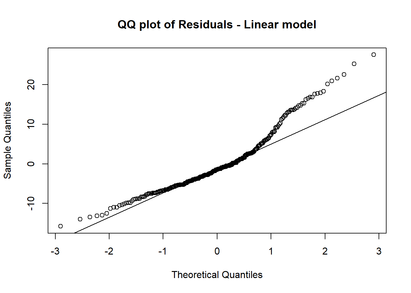

qqnorm(residuals(mixed_model),main="QQ plot of Residuals - Mixed model")
qqline(residuals(mixed_model))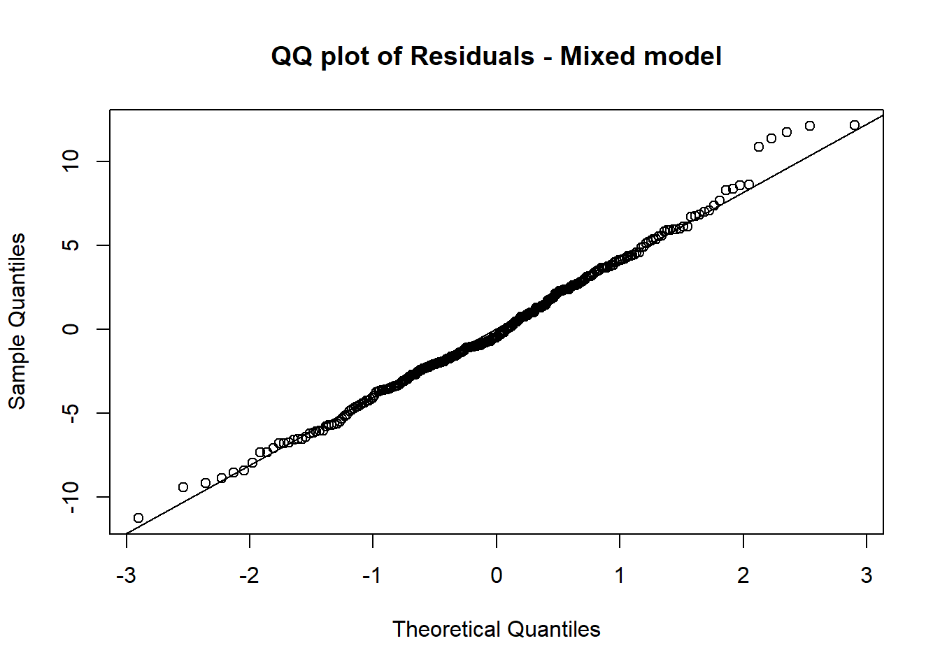

The mixed model satisfied the normality assumption much better as the points are closer to the line on the QQ Plot.

12.1.6 f. (7510 only) Examine the BLUPs from the mixed model in (d). Do you notice any patterns?

library(lme4)
ranef(mixed_model)$replicate

## NULL

ranef(mixed_model)$recipe

##     (Intercept)
## A -3.077238e-14
## B -4.667144e-14
## C -2.051492e-14

The number seems to be close to 0.

#??? what patten central point?variance or intercept?
#??? why replicate null? 
#!!! Alternative solution: with nested structure for HW3. replication is nested within recipe.???

12.2 2) The purpose of random effects is to remove variation from known sources. In this problem, we will use this idea and see how it can work with a popular technique for predictive modeling, the random forest. Random forests were covered in the prerequisite course, and can be fit using the randomForest function in the randomForest library. The dataset Problem-2.csv has a simulated dataset. There is a nonlinear relationship between 6 numeric explanatory variables x1, . . . x6 and the response y, to addition to a grouping effect according to the ID variable, which has 100 levels.

set.seed(1)
Problem2 <- read.csv("E:/Cloud/OneDrive - University of Missouri/Mizzou_PhD/Class plan/Applied Stats Model II/HW3/Problem-2.csv", stringsAsFactors = TRUE)

12.2.1 a. Read in the dataset, and split the data into a training and test set, using 95% of the data for the training set. Set a seed of 1 for consistency of results.

train=sample(1:nrow(Problem2), nrow(Problem2)*0.95)
Problem2.train = Problem2[train,]
Problem2.test = Problem2[-train,]

12.2.2 b. Fit a random forest model to the training data using y as the response with x1, . . . x6 and ID as the explanatory variables. Use the model to predict y in the test set and compute the test root mean squared error ( RMSE ).

#install.packages("randomForest")
library(randomForest)

## randomForest 4.7-1

## Type rfNews() to see new features/changes/bug fixes.

## 
## Attaching package: 'randomForest'

## The following object is masked from 'package:dplyr':
## 
##     combine

## The following object is masked from 'package:ggplot2':
## 
##     margin

RF_model =randomForest(y~x1+x2+x3+x4+x5+x6+ID,data=Problem2,subset=train,importance=TRUE)

Problem2.test$y_RF <- predict(RF_model,newdata=Problem2.test)

sqrt(sum((Problem2.test$y_RF - Problem2.test$y)^2)/175)

## [1] 4.503223

The RMSE is 4.5

12.2.3 c. Fit the mixed model yij = µ + IDi + εij to the training data. This model does not use the x_i at all, and has a random intercept based on ID. After fitting the model, extract the BLUPs for ID and add them to the constant µˆ, the estimate of the overall intercept. What do these values represent? Store them in a data frame along with a column storing the IDs.

P2_mixed_model <- lmer(y ~ 1 + (1 | ID), Problem2.train)
summary(P2_mixed_model)

## Linear mixed model fit by REML ['lmerMod']
## Formula: y ~ 1 + (1 | ID)
##    Data: Problem2.train
## 
## REML criterion at convergence: 21249.3
## 
## Scaled residuals: 
##     Min      1Q  Median      3Q     Max 
## -2.9799 -0.6991 -0.0011  0.7052  3.2476 
## 
## Random effects:
##  Groups   Name        Variance Std.Dev.
##  ID       (Intercept)  7.018   2.649   
##  Residual             32.786   5.726   
## Number of obs: 3325, groups:  ID, 100
## 
## Fixed effects:
##             Estimate Std. Error t value
## (Intercept)  24.5945     0.2829   86.92

#P2_ID_BLUP = ranef(P2_mixed_model)$ID
library(tidyverse)

#S23:

#predict(mixed_model, newdata=data.frame(operator="a"))

Problem2.test$BLUP <- predict(P2_mixed_model, newdata=Problem2.test)

DF_BLUPx <- fixef(P2_mixed_model) + ranef(P2_mixed_model)$ID
DF_BLUPx$ID <- 1:nrow(DF_BLUPx)

The values represent the intercept for each ID.

12.2.4 d. Add a column to the test dataset containing the values obtained in part c, joined to the test dataset by matching the IDs. Note: with the dplyr package loaded, you can quickly join by ID using a line like: Data.Test <- left_join(Data.Test, int_plus_blups, by = “ID”) Examine the first few rows and describe what the new column represents.

Problem2.test <- left_join(Problem2.test, DF_BLUPx, by = "ID")

The new column represents the intercept for each ID in the test dataset.

12.2.5 e. Compute the residuals of the mixed model fit in (c) using the residuals() function, store them in a column of the training data.

Problem2.train$residualx = residuals(P2_mixed_model)

12.2.6 f. Fit another random forest model to the training data, using the residuals from part (e) as the response and only x1, . . . x6 as the explanatory variables. Use this model to predict into the test data and store these predictions. What do these predictions represent?

#why I cannot use subset anymore??? diff dataaset?
RF_residuals_model =randomForest(residualx~x1+x2+x3+x4+x5+x6,data=Problem2.train,importance=TRUE)

Problem2.test$y_RF_residual <- predict(RF_residuals_model,newdata=Problem2.test)

The prediction represents the additional variations beyond the ID’s variation.

12.2.7 g. Add the predictions in (f) to the values joined to the test data in (d). Consider these values test predictions, and compute the test MSE. Compare this to the test MSE compared in part (b). What do you observe?

sqrt(sum((Problem2.test$BLUP + Problem2.test$y_RF_residual - Problem2.test$y)^2)/175)

## [1] 3.608027

(3.6-4.5)/4.5

## [1] -0.2

The RMSE is reduced from 4.5 to 3.6 or a 20% reduction. The model’s prediction is greatly improved.