Chapter 8 Question 2
2) Ordinal Regression The DrugConsumption.csv file on Canvas contains records for 1458 respondents. For each respondent 12 attributes are known: Personality measurements which include NEO-FFI-R (neuroticism, extraversion, openness to experience, agreeableness, and conscientiousness), BIS-11 (impulsivity), and ImpSS (sensation seeking), level of education, age, gender and country of residence. In addition, participants were questioned concerning their use of 18 legal and illegal drugs, of which only LSD is included for our study. The variables are as follows: • LSD: Target variable, ordinal with levels CL0-CL5, which correspond to “Never Used,” “Used over a Decade Ago,” “Used in Last Decade,” “Used in Last Year,” “Used in Last Month,” “Used in Last Week.” • Age: Categorical age • Gender: Gender • Education: Categorical Educational level • Country: UK or USA • Nscore: NEO-FFI-R, a psychological measure of Neuroticism • Escore: NEO-FFI-R Extraversion. • Oscore: NEO-FFI-R Openness to experience • Ascore: NEO-FFI-R Agreeableness • Cscore: NEO-FFI-R Conscientiousness • Impulsive: Impulsiveness score measured by BIS-11 • SS: Impulsive Sensation Seeking measured by ImpSS You may read the data as follows: Drugs <- read.csv(“…/DrugConsumption.csv,” stringsAsFactors = TRUE) Drugs$LSD <- ordered(Drugs$LSD,levels = c(paste0(“CL,”0:5)))
Drugs <- read.csv("E:/Cloud/OneDrive - University of Missouri/Mizzou_PhD/Class plan/Applied Stats Model II/HW1/DrugConsumption.csv", stringsAsFactors = TRUE) #install.packages("tidyverse")
library(tidyverse) # for mutate function#??? the following code gave me error. What is it?
#Drugs$LSD <- ordered(Drugs$LSD,levels = c(paste0("CL",0:5)))8.1 a. (5 points) Make a plot or set of tables showing the distribution of LSD use between genders and interpret. You can use code similar to that on slide 84 of the course notes.
I re-coded the categories into descriptive names “Used over a Decade Ago,” “Used in Last Decade,” “Used in Last Year,” “Used in Last Month,” “Used in Last Week.”
Based on the plot, male are more likely to use drugs than female. Many female never used any drugs.
Drugs$LSD_o <- NA
Drugs$LSD_o[Drugs$LSD %in%c("CL0")] <- "Never Used"
Drugs$LSD_o[Drugs$LSD %in%c("CL1")] <- "Used over a Decade Ago"
Drugs$LSD_o[Drugs$LSD %in%c("CL2")] <- "Used in Last Decade"
Drugs$LSD_o[Drugs$LSD %in%c("CL3")] <- "Used in Last Year"
Drugs$LSD_o[Drugs$LSD %in%c("CL4")] <- "Used in Last Month"
Drugs$LSD_o[Drugs$LSD %in%c("CL5")] <- "Used in Last Week"
table(Drugs$LSD_o)
##
## Never Used Used in Last Decade Used in Last Month
## 866 134 62
## Used in Last Week Used in Last Year Used over a Decade Ago
## 40 146 210Plot_DF <- Drugs |>
group_by(Gender, LSD_o) |>
summarise(count=n()) |>
group_by(Gender) |>
mutate(etotal=sum(count), proportion=count/etotal)## `summarise()` has grouped output by 'Gender'. You can override using the
## `.groups` argument.# mutate(Age_Grp=cut_number(age,4)) |> not used since the gender is not continous.# Plot_DF -> only a dataframe
Gender_Plot <- ggplot(Plot_DF, aes(x=Gender, y=proportion,
group=LSD_o, linetype=LSD_o))+
geom_line()
Gender_Plot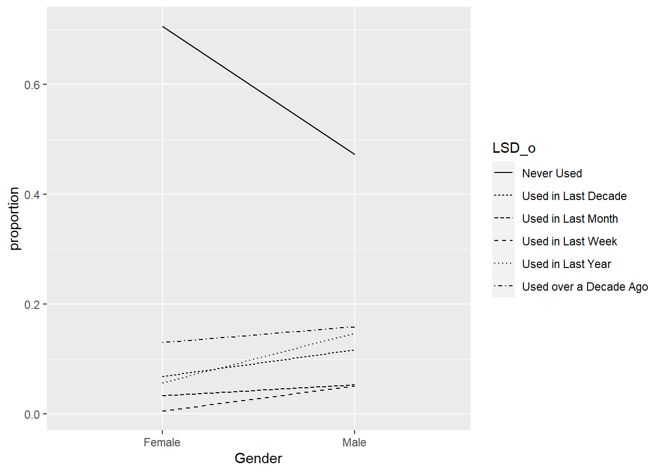
8.2 b. (9 points) Fit a proportional odds model using LSD as the response variable and the other variables listed above as predictors. Using drop1(), test if the variables are significant or insignificant and describe 2 your results.
The significant variables are age 55+, GenderMale, CountryUSA, Oscore and Cscore.
The drop1 function shows gender, country, Oscore and Cscore are significant but not the age 55+. Strangely the drop1 function doesn’t factorize the categorical variables such as age and education.
Overall, the two results are quite consistent with each other.
library(MASS)##
## Attaching package: 'MASS'## The following object is masked from 'package:dplyr':
##
## selectDrugs$LSD_o <- ordered(Drugs$LSD_o,
levels=c("Never Used", "Used over a Decade Ago", "Used in Last Decade", "Used in Last Year", "Used in Last Month", "Used in Last Week"))
PropOdds_Model <- MASS::polr(LSD_o ~ Age + Gender + Education + Country + Nscore + Escore + Oscore + Ascore + Cscore, Drugs)
summary(PropOdds_Model)##
## Re-fitting to get Hessian## Call:
## MASS::polr(formula = LSD_o ~ Age + Gender + Education + Country +
## Nscore + Escore + Oscore + Ascore + Cscore, data = Drugs)
##
## Coefficients:
## Value Std. Error t value
## Age25-34 -0.097001 0.16037 -0.60486
## Age35-44 -0.006247 0.17504 -0.03569
## Age45-54 -0.218738 0.18630 -1.17412
## Age55+ -0.671385 0.26083 -2.57408
## GenderMale 0.773020 0.12094 6.39159
## EducationHighSchool -0.105167 0.29551 -0.35588
## EducationHSDropout 0.124446 0.22553 0.55180
## EducationPostGraduate -0.294833 0.17637 -1.67163
## EducationProfessionalCert 0.011469 0.19528 0.05873
## EducationSomeCollege 0.078480 0.16218 0.48392
## CountryUSA 1.708138 0.13773 12.40252
## Nscore -0.110185 0.06866 -1.60469
## Escore 0.014487 0.06745 0.21478
## Oscore 0.597784 0.06685 8.94237
## Ascore -0.018913 0.05870 -0.32221
## Cscore -0.178554 0.06696 -2.66662
##
## Intercepts:
## Value Std. Error t value
## Never Used|Used over a Decade Ago 1.2133 0.1750 6.9337
## Used over a Decade Ago|Used in Last Decade 2.1296 0.1832 11.6275
## Used in Last Decade|Used in Last Year 2.9048 0.1887 15.3969
## Used in Last Year|Used in Last Month 4.1597 0.2054 20.2562
## Used in Last Month|Used in Last Week 5.2439 0.2415 21.7105
##
## Residual Deviance: 3143.917
## AIC: 3185.917#problen with converge if I include the same variable LSD. need to remove it.drop1(PropOdds_Model,test="Chisq")## Single term deletions
##
## Model:
## LSD_o ~ Age + Gender + Education + Country + Nscore + Escore +
## Oscore + Ascore + Cscore
## Df AIC LRT Pr(>Chi)
## <none> 3185.9
## Age 4 3186.2 8.270 0.082171 .
## Gender 1 3225.3 41.410 1.234e-10 ***
## Education 5 3181.0 5.122 0.401142
## Country 1 3343.6 159.732 < 2.2e-16 ***
## Nscore 1 3186.5 2.573 0.108671
## Escore 1 3184.0 0.046 0.829943
## Oscore 1 3266.8 82.918 < 2.2e-16 ***
## Ascore 1 3184.0 0.104 0.747364
## Cscore 1 3191.1 7.183 0.007359 **
## ---
## Signif. codes: 0 '***' 0.001 '**' 0.01 '*' 0.05 '.' 0.1 ' ' 1# drop1(PropOdds_Model)
# why is the age not broken down as factors?
# Drop1 will drop all in age variable. 8.3 c. (6 points) Interpret the values of the intercepts θj .
The intercepts are listed as below:
Never Used|Used over a Decade Ago 3.364569 . It means cumulative odds of being never used is 3.36 when all other variables are set to 0.
Used over a Decade Ago|Used in Last Decade 8.411502 It means cumulative odds of being Used in last decade is 8.411502 when all other variables are set to 0.
Used in Last Decade|Used in Last Year 18.26159 It means cumulative odds of being Used in last year is 18.2615 when all other variables are set to 0.
Used in Last Year|Used in Last Month 64.0523 It means cumulative odds of being Used in last month is 64.0523 when all other variables are set to 0.
Used in Last Month|Used in Last Week 189.4074 It means cumulative odds of being Used in last week is 189 when all other variables are set to 0.
PropOdds_Model_sum <- summary(PropOdds_Model)##
## Re-fitting to get Hessian#PropOdds_Model_sum$coefficients
exp(1.2133)## [1] 3.364569exp(2.1296)## [1] 8.411502exp(2.9048)## [1] 18.26159exp(4.1597)## [1] 64.0523exp(5.2439)## [1] 189.4074#!not sure how to explain it. S97. Does it also needs a exp()? -> how to extract it automatically? does it mean % of ppl???8.4 d. (10 points) Print the coefficient table and interpret the values of the significant personality characteristics.
The open to experience increase the odds of using the drugs by 1.81.
Conscientiousness decreases the odds of using the drugs by 0.8.
coefficients(PropOdds_Model)## Age25-34 Age35-44 Age45-54
## -0.097000990 -0.006246867 -0.218738114
## Age55+ GenderMale EducationHighSchool
## -0.671384707 0.773019582 -0.105166700
## EducationHSDropout EducationPostGraduate EducationProfessionalCert
## 0.124446396 -0.294833364 0.011469188
## EducationSomeCollege CountryUSA Nscore
## 0.078480163 1.708138461 -0.110184787
## Escore Oscore Ascore
## 0.014486532 0.597783608 -0.018912601
## Cscore
## -0.178553588#??? are the coefficient intercept or beta?
#Both personality significant. The higher the less likely to move ?!!!
#Oscore
exp(0.597784) ## [1] 1.818085#Cscore
exp(-0.178554)## [1] 0.83647898.5 e. (7250 only) (6 points) Explore interacting some of the categorical demographic variables with the personality measurements and report your findings, does the nature of any personality characteristics affect on LSD usage change according to your analysis?
I tested the interaction between demographic variables (age, gender and education) and personality measurements (Oscore, Cscore).
I found the following significant interactions:
Age35-44:Oscore -0.396513
Age25-34:Cscore -0.368074
Age35-44:Cscore -0.590439
Age45-54:Cscore -0.587787
Age55+:Cscore -0.614652
The results have a consistent theme that more mature people (age above 18-24) and higher on open to experience or conscientiousness scores are less likely to use drugs.
PropOdds_Model_int <- MASS::polr(LSD_o ~ Age + Gender + Education + Country + Nscore + Escore + Oscore + Ascore + Cscore + Age*Oscore + Age*Cscore + Gender*Oscore + Gender*Cscore + Education*Oscore + Education *Cscore, Drugs)
summary(PropOdds_Model_int)
##
## Re-fitting to get Hessian## Call:
## MASS::polr(formula = LSD_o ~ Age + Gender + Education + Country +
## Nscore + Escore + Oscore + Ascore + Cscore + Age * Oscore +
## Age * Cscore + Gender * Oscore + Gender * Cscore + Education *
## Oscore + Education * Cscore, data = Drugs)
##
## Coefficients:
## Value Std. Error t value
## Age25-34 -0.172081 0.17273 -0.99623
## Age35-44 -0.104423 0.18315 -0.57016
## Age45-54 -0.280105 0.19515 -1.43533
## Age55+ -0.654289 0.26780 -2.44318
## GenderMale 0.774285 0.12648 6.12198
## EducationHighSchool 0.019760 0.32261 0.06125
## EducationHSDropout -0.102915 0.24983 -0.41194
## EducationPostGraduate -0.306062 0.19143 -1.59878
## EducationProfessionalCert 0.046031 0.20393 0.22572
## EducationSomeCollege 0.070706 0.17446 0.40528
## CountryUSA 1.744167 0.14162 12.31579
## Nscore -0.118884 0.06971 -1.70541
## Escore 0.038420 0.06843 0.56143
## Oscore 0.685866 0.17126 4.00483
## Ascore -0.018826 0.06047 -0.31131
## Cscore 0.116770 0.16389 0.71247
## Age25-34:Oscore 0.004876 0.17067 0.02857
## Age35-44:Oscore -0.396513 0.17969 -2.20666
## Age45-54:Oscore -0.143649 0.21006 -0.68386
## Age55+:Oscore -0.227344 0.27432 -0.82876
## Age25-34:Cscore -0.368074 0.16557 -2.22312
## Age35-44:Cscore -0.590439 0.17650 -3.34527
## Age45-54:Cscore -0.587787 0.19676 -2.98727
## Age55+:Cscore -0.614652 0.29484 -2.08467
## GenderMale:Oscore 0.009991 0.12113 0.08248
## GenderMale:Cscore -0.052592 0.12510 -0.42040
## EducationHighSchool:Oscore -0.293782 0.27753 -1.05855
## EducationHSDropout:Oscore -0.255640 0.25420 -1.00565
## EducationPostGraduate:Oscore 0.058642 0.19749 0.29693
## EducationProfessionalCert:Oscore 0.303077 0.21251 1.42618
## EducationSomeCollege:Oscore 0.012843 0.16599 0.07737
## EducationHighSchool:Cscore 0.056019 0.32688 0.17138
## EducationHSDropout:Cscore -0.226221 0.24937 -0.90717
## EducationPostGraduate:Cscore 0.254668 0.19192 1.32694
## EducationProfessionalCert:Cscore 0.101606 0.21581 0.47082
## EducationSomeCollege:Cscore 0.026077 0.16748 0.15571
##
## Intercepts:
## Value Std. Error t value
## Never Used|Used over a Decade Ago 1.1821 0.1815 6.5142
## Used over a Decade Ago|Used in Last Decade 2.1166 0.1893 11.1805
## Used in Last Decade|Used in Last Year 2.9087 0.1952 14.9009
## Used in Last Year|Used in Last Month 4.1936 0.2136 19.6321
## Used in Last Month|Used in Last Week 5.2923 0.2499 21.1740
##
## Residual Deviance: 3108.449
## AIC: 3190.449STAT 4520/7520 - Homework 2 Spring 2022 Due: March 6, 2022 The French Motor Third-Party Liability Claims dataset is located in Insurance.csv and contains records on insurance policies. A claim is the request made by a policyholder to the insurer to compensate for a loss covered by the insurance. Insurance companies are interested in modeling how much they are expected to payout per year. In other words the mean of the total claim amount per year also referred to as the “pure premium.” The varibles in the dataset are as follows: “Feature” variables: • Area: The area code. • VehPower: The power of the car (ordered categorical but treat as numeric). • VehAge: The vehicle age, in years. • DrivAge: The driver age, in years. • BonusMalus: Bonus/malus, between 50 and 350 and relating to the carbon emissions of the vehicle: < 100 means bonus(tax credit), > 100 means malus(tax penalty). • VehBrand: The car brand (unknown categories). • VehGas: The car gas, Diesel or regular. • Density: The (log of) density of inhabitants (number of inhabitants per km2) in the city the driver of the car lives in. • Region: The policy regions in France (based on a standard French classification). “Target” variables: • ClaimNb: Total number of claims on the policy. • Exposure: Number of years the policy has been held. • Frequency: Average number of claims per year on the policy. • AvgClaimAmount: Average amount paid out per claim in the policy. • PurePremium: Expected total claim amount per year for each policy.
There are several ways to create these predictions, we could: 1. Model the number of claims with a count model, and separately the average claim amount per claim and multiply the predictions of both in order to get the total claim amount. 2. Model the total claim amount per exposure directly, typically with a Tweedie distribution. We will explore both of these options here. The dataset can be loaded for properly formatted with the commands:
Insurance <- read.csv("E:/Cloud/OneDrive - University of Missouri/Mizzou_PhD/Class plan/Applied Stats Model II/HW2/Insurance.csv", stringsAsFactors = TRUE)
Insurance$VehBrand <- as.factor(Insurance$VehBrand)
Insurance$VehPower <- as.factor(Insurance$VehPower)
Insurance$VehGas <- as.factor(Insurance$VehGas)
Insurance$Region <- as.factor(Insurance$Region)
Insurance$Area <- as.factor(Insurance$Area)