Chapter 11 3. Tweedie
11.1 a. (8 points) Using the entire dataset, create a profile likelihood of the index values p for use in a glm utilizing the Tweedie distribution to predict PurePremium directly. Make a plot of the profile likelihood and select the best value. (7520 - 3 points): For graduate students, I expect some exploration to find the best value as these data are quite poorly behaved. Look at the “Value” section of ?tweedie.profile for some hints, and I would suggest narrowing the search space for p and evaluating it on a somewhat fine grid.
library(tweedie)
?tweedie.profile
## starting httpd help server ... done#per tweedie documentation on p.vec. if there is 0, below is the recommendated setting.
TW_p_log <- tweedie.profile(AvgClaimAmount ~ .,
p.vec = seq(from=1.2,to=1.8,by=0.1),
link.power = 0, do.plot = TRUE,# log link
data=Insurance)## 1.2 1.3 1.4 1.5 1.6 1.7 1.8
## .......Done.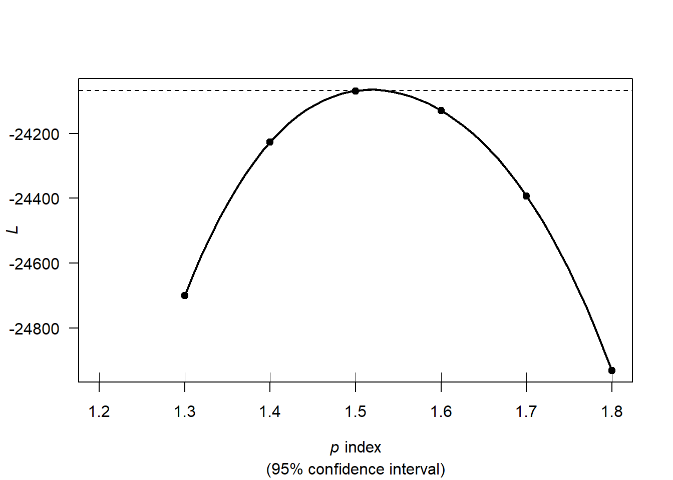
TW_p_log <- tweedie.profile(AvgClaimAmount ~ .,
p.vec = seq(from=1.4,to=1.7,by=0.05),
link.power = 0, do.plot = TRUE,# log link
data=Insurance)
## 1.4 1.45 1.5 1.55 1.6 1.65 1.7
## .......Done.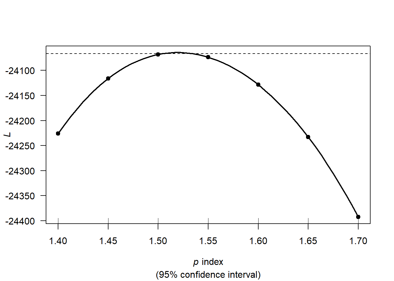
Tweedie_p_log = TW_p_log$p.max
Tweedie_p_log
## [1] 1.522449The best value is 1.52.
11.2 b. Fit the Tweedie GLM model using the optimal power value you computed from the previous question. The file Insurance_test.csv contains a few additional observations which were not a portion of the data used to fit the previous models. We can read it in and format it using syntax similar to when we started. NewDataPoints <- read.csv(“…./Insurance_test.csv”) NewDataPoints$VehBrand <- as.factor(NewDataPoints$VehBrand) NewDataPoints$VehPower <- as.factor(NewDataPoints$VehPower) NewDataPoints$VehGas <- as.factor(NewDataPoints$VehGas) NewDataPoints$Region <- as.factor(NewDataPoints$Region) NewDataPoints$Area <- as.factor(NewDataPoints$Area)
NewDataPoints <- read.csv("E:/Cloud/OneDrive - University of Missouri/Mizzou_PhD/Class plan/Applied Stats Model II/HW2/Insurance_test.csv")
NewDataPoints$VehBrand <- as.factor(NewDataPoints$VehBrand)
NewDataPoints$VehPower <- as.factor(NewDataPoints$VehPower)
NewDataPoints$VehGas <- as.factor(NewDataPoints$VehGas)
NewDataPoints$Region <- as.factor(NewDataPoints$Region)
NewDataPoints$Area <- as.factor(NewDataPoints$Area)library(statmod) # For tweedie family in glm()
clot_Tweedie_log <- glm(AvgClaimAmount ~ ., data=Insurance,
family=tweedie(var.power=TW_p_log$p.max,link.power=0))summary(clot_Tweedie_log)##
## Call:
## glm(formula = AvgClaimAmount ~ ., family = tweedie(var.power = TW_p_log$p.max,
## link.power = 0), data = Insurance)
##
## Deviance Residuals:
## Min 1Q Median 3Q Max
## -143.413 -2.577 -2.358 -2.138 88.120
##
## Coefficients: (1 not defined because of singularities)
## Estimate Std. Error t value Pr(>|t|)
## (Intercept) -1.636e+00 2.401e-01 -6.814 9.62e-12 ***
## ClaimNb 5.551e+00 2.373e-02 233.891 < 2e-16 ***
## Exposure -4.523e-01 6.460e-02 -7.002 2.56e-12 ***
## AreaB -6.157e-01 9.202e-02 -6.691 2.25e-11 ***
## AreaC -9.969e-01 1.217e-01 -8.193 2.62e-16 ***
## AreaD -1.432e+00 1.886e-01 -7.592 3.21e-14 ***
## AreaE -1.863e+00 2.469e-01 -7.547 4.54e-14 ***
## AreaF -2.206e+00 3.625e-01 -6.086 1.17e-09 ***
## VehPower5 1.935e-01 7.206e-02 2.685 0.007252 **
## VehPower6 1.713e-01 6.842e-02 2.504 0.012298 *
## VehPower7 -1.871e-01 6.894e-02 -2.713 0.006662 **
## VehPower8 -1.024e-01 1.057e-01 -0.968 0.332876
## VehPower9 3.152e-01 1.066e-01 2.958 0.003098 **
## VehPower10 4.430e-01 1.133e-01 3.910 9.23e-05 ***
## VehPower11 7.907e-01 1.423e-01 5.556 2.78e-08 ***
## VehPower12 6.662e-01 2.117e-01 3.146 0.001654 **
## VehPower13 1.599e-01 2.723e-01 0.587 0.557015
## VehPower14 -2.349e+00 6.682e-01 -3.515 0.000441 ***
## VehPower15 9.716e-01 4.146e-01 2.344 0.019100 *
## VehAge -3.288e-03 4.003e-03 -0.821 0.411487
## DrivAge 1.230e-02 1.488e-03 8.271 < 2e-16 ***
## BonusMalus 7.315e-03 1.185e-03 6.171 6.84e-10 ***
## VehBrandB10 7.370e-02 1.421e-01 0.519 0.603970
## VehBrandB11 7.272e-01 1.379e-01 5.275 1.33e-07 ***
## VehBrandB12 -4.509e-01 9.113e-02 -4.948 7.54e-07 ***
## VehBrandB13 1.093e+00 1.305e-01 8.376 < 2e-16 ***
## VehBrandB14 6.719e-01 2.192e-01 3.064 0.002182 **
## VehBrandB2 9.120e-02 5.343e-02 1.707 0.087828 .
## VehBrandB3 -7.350e-02 7.786e-02 -0.944 0.345144
## VehBrandB4 3.675e-01 1.017e-01 3.614 0.000302 ***
## VehBrandB5 4.190e-01 8.288e-02 5.055 4.33e-07 ***
## VehBrandB6 3.926e-01 8.891e-02 4.416 1.01e-05 ***
## VehGasRegular -2.223e-01 4.420e-02 -5.028 4.97e-07 ***
## Density 3.520e-01 4.718e-02 7.460 8.80e-14 ***
## RegionR21 6.821e-01 4.580e-01 1.489 0.136462
## RegionR22 3.816e-01 2.036e-01 1.875 0.060840 .
## RegionR23 6.810e-01 3.349e-01 2.034 0.041990 *
## RegionR24 7.622e-01 1.072e-01 7.107 1.20e-12 ***
## RegionR25 2.417e-02 1.975e-01 0.122 0.902627
## RegionR26 5.522e-01 2.320e-01 2.380 0.017305 *
## RegionR31 8.848e-01 1.478e-01 5.986 2.16e-09 ***
## RegionR41 -3.213e-02 1.409e-01 -0.228 0.819610
## RegionR42 7.103e-02 2.552e-01 0.278 0.780753
## RegionR43 1.662e-01 7.882e-01 0.211 0.832964
## RegionR52 4.081e-01 1.255e-01 3.250 0.001153 **
## RegionR53 7.129e-01 1.176e-01 6.061 1.36e-09 ***
## RegionR54 -7.083e-02 1.370e-01 -0.517 0.605221
## RegionR72 5.431e-02 1.322e-01 0.411 0.681283
## RegionR73 6.923e-01 2.178e-01 3.179 0.001479 **
## RegionR74 -6.384e-01 1.781e-01 -3.585 0.000337 ***
## RegionR82 6.612e-01 1.075e-01 6.150 7.83e-10 ***
## RegionR83 -8.528e-02 4.404e-01 -0.194 0.846456
## RegionR91 5.483e-01 1.659e-01 3.305 0.000949 ***
## RegionR93 8.103e-01 1.147e-01 7.065 1.63e-12 ***
## RegionR94 -2.268e-01 5.804e-01 -0.391 0.695913
## PurePremium 3.061e-07 1.992e-08 15.364 < 2e-16 ***
## Frequency 2.106e-02 1.861e-03 11.320 < 2e-16 ***
## Predicted_Class -1.096e+00 4.752e-01 -2.307 0.021053 *
## Predicted_Class_NB NA NA NA NA
## ---
## Signif. codes: 0 '***' 0.001 '**' 0.01 '*' 0.05 '.' 0.1 ' ' 1
##
## (Dispersion parameter for Tweedie family taken to be 52.21709)
##
## Null deviance: 2712009 on 44998 degrees of freedom
## Residual deviance: 620930 on 44941 degrees of freedom
## AIC: NA
##
## Number of Fisher Scoring iterations: 20